Posts

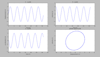
IDEAL SIMPLE HARMONIC OSCILLATOR-EULER METHOD
Image
from pylab import * n=100 x=zeros(n,dtype='float') t=zeros(n,dtype='float') v=zeros(n,dtype='float') a=zeros(n,dtype='float') x[0],v[0],w=0,2,1 dt=10*pi/(w*n) a[0]=-w*w*x[0] for i in range(1,n):     a[i]=-w*w*x[i-1]     v[i]=v[i-1]+a[i]*dt     x[i]=x[i-1]+v[i]*dt     t[i]=t[i-1]+dt subplot(2,2,1) title('t - x plot') xlabel(' time (t)') ylabel('displacement (x)') plot(t,x) subplot(2,2,2) title('t- v plot') xlabel('time (t)') ylabel('velocity (v)') plot(t,v) subplot(2,2,3) title('t- a plot') xlabel('time (t)') ylabel('acceleration (a)') plot(t,a) subplot(2,2,4) axis('equal') title('phase space plot') xlabel('displacement (x)') ylabel('velocity (v)') plot(x,v) show() OUTPUT  

SHO-Feynman Newton Method

Image
#Ideal simple Harmonic Oscillator #Harmonic oscillator #dx/dt=v #dv/dt=-w*w*x #Feynman-Newton method #x(t+h)=x(t)+h*v(t+h/2) #v(t+h/2)=v(t-h/2)+h*a(t) #v(1/2)=v0+(h/2)a0 from pylab import* from math import* x0=5 v0=5 w=1 t=0 #initial time h=0.001 #time step size xdat=[] vdat=[]#velocity data store here time=[]#time stored here v0=v0+h*(-w*w*x0)/2 while(t<=100):     x1=x0+h*v0     v1=v0+h*(-w*w*x1)           xdat.append(x1)     vdat.append(v1)     time.append(t)     x0=x1     v0=v1     t=t+h    figure(1) title("Harmonic oscillator motion") xlabel(" Time") ylabel("x") plot(time,xdat) grid(True) figure(2) title("Harmonic oscillator motion") xlabel("Time") ylabel("Velocity") plot(time,vdat) grid(True) figure(3) title("Harmonic oscillator motion") xlabel("x") ylabel("Velocity") plot(xdat,vdat) grid(True) show() output #DAMPED...

Planetary Motion

Image
#Planetary Motion Program 1  from pylab import* gm=10.0 x=20.0 y=0.0 r=sqrt(x*x+y*y) #velocity=sqrt(gm/r), we get circular path # for less or more velocities we get elliptical or hyperbolic path f=1 #choose different f values, for example f=0.8, 1.0, 1.2, 1.4 ,see difference vx=0 vy=f*sqrt(gm/r) h=0.05 xpos=[x] ypos=[y] for i in range(30000):     r=(x*x+y*y)**0.5     vx=vx-(gm*x*h/(r*r*r))     vy=vy-(gm*y*h/(r*r*r))     x=x+vx*h     y=y+vy*h     xpos.append(x)     ypos.append(y) plot(xpos,ypos,'.b') xlabel('x') ylabel('Y') axis('equal') show()  Out put   #-------------------PLANETARY MOTION program 2--------------------------# #Gravitation is a conservative fore: E = T + V #The total energy of the system can be expressed as two coupled 1st order odes: #dr/dt = v              Where v is the veloc...

Radio active decay-Monte Carlo Method

Image
# Radio active decay from pylab import* from random import * n,Lambda,t,tm=1000000,0.2,0.0,10 N=[n] T=[t] while n>0 and t<tm:     for i in range(n):         if random()<=Lambda:             n-=1     t+=1     N.append(n)     T.append(t) plot(T,N,'r') T=array(T) Y=N[0]*exp(-Lambda*T) plot(T,Y,'b') legend(['simulated','exponential']) show() output

Value of Pi

Image
Theory value of Pi is calculated using the Monte Carlo method - generate a large number of random points and see how many fall in the circle enclosed by the unit square.    # Program from random import * j=0 for i in range(10000000):     x=random()     y=random()     if (x**2+y**2)<=1:j+=1 print "Value of pi = ",4.0*j/i

Body falling in a viscous medium using Euler method

Image
Theory Weight of body Mg=density*g*Volume Upward thrust=Volume*d2*g resultant downward force=V*d1*g-V*d2*g Program: #Simulation of a body falling in a viscous medium using Euler method #Falling of a body through viscous medium #Loss of weight   V*d1*g-V*d2*g=V*d1*g(1-d2/d1)=m*a where a=g(1-d2/d1) #Drag in the case of ball 6*pi*eta*a*v=k*v #dy/dt=v #dv/dt=a-kv from pylab import* from math import* d1=2000.0 #density of body d2=750.0 #density of liquid g=9.8 height=2000 y0=0 v0=0 a=(1.0- d2/d1)*g #including buoyant force k=0.2 #drag coefficient h=0.001 t=0 y=[y0] v=[v0] time=[t] while height-y0>0:     v1=v0+h*(a-k*v0)     y1=y0+h*v0      t=t+h     y.append(height-y1)     v.append(fabs(v1))     time.append(t)     y0=y1     v0=v1 figure(1) title("Fall through viscous medium") xlabel(" Time") ylabel("Position") plot...

Free fall of a body from a height

Image
#Free Fall-Euler Method neglect air resistance from pylab import* t,v=0,0 #initialise the values g=-9.8 dt=0.01 h=input('Enter the height of fall: ')tdat,hdat,vdat,gdat=[],[],[],[] print 'time\theight\tvelocity\tacceleration\t' while h>=0:     a=g     v+=a*dt     h+=v*dt     t+=dt     tdat.append(t)     hdat.append(h)     vdat.append(v)     gdat.append(a)     print '%10.3f\t%10.3f\t%10.3f\t%10.3f\t'%(t,h,v,a) subplot(1,3,1) title('position-time') plot(tdat,hdat) subplot(1,3,2) plot(tdat,vdat) title('Velocity-time') subplot(1,3,3) title('Acceleration-time') plot(tdat,gdat) show()     #Free Fall-Euler Method with air resistance from pylab import* t,v=0,0 #initialise the values g=-9.8 dt=0.01 h=input('Enter the height of fall: ') tdat,hdat,vdat,gdat=[],[],[],[] print 'time\theight\tvelocity\taccel...